Unless a problem has a number of the form "B.m.n", or it is otherwise stated, the problem is from the text. Many of the answers are in the back of the text.
The problems are not quite the same in the regular 4th edition and the 4th international edition. I will take that into account when assigning them.
If a problem has a number of the form "B.m.n", then it is to be found on Canvas.
This page started as a copy of last year's. Therefore it may change in the course of the quarter. Do not consider a saved version valid in the future.
It should be understood that the problems in last year's mid-quarter and final exams, posted on Canvas, should be considered assigned homework problems before each of this year's exams.
September 25. 2.1.
September 28. 2.2, 2.3. In 2.2 ω is a constant. I think 4f, rather than 2ω, belongs in front but that won't effect the answers to the problem. By the "impulse response" is meant the output y() = g() that results when the input u(t) = δ(t) ∀ t.
September 30. 2.5 (assume a linear causal system), 2.6.
October 2. 2.9. This problem is something of a joke because, since there is a current source on the left, the transfer function is simply the impedance of the RLC circuit on the right. However you should do it as posed: find the state/output equations and then compute the transfer function from them. I regret the author's predilection for circuit elements of value 1.
October 5. 2.14, 2.15.
October 7. Problems B2.14, B2.17, available on Canvas.
October 9. 3.1,3.2,3.3,3.5 (3.6 in the international edition) You should have downloaded my table of Jordan forms, from Canvas, for later use.
October 12. 3.6,3.7,3.8 (3.7,3.12,3.13 in the international edition).
October 14. 3.12, 3.13 (3.17,3.18 in international edition).
October 16. 3.18 (3.23 in the inernational edition). Also do for A3 of problem 3.13 (3.18 in the internatioal edition) and for the matrix
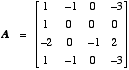
That A is in the table of Jordan forms, which you should use when possible.
October 19. 3.21 (3.26 in the international edition).
October 21. B.3.21. Do 3.22 (3.27 in the international edition) but using rather the matrix
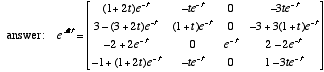
You should find my table of Jordan forms useful for this problem.
That is the last homework assignment before the mid-quarter exam on Oct. 28, which will be based mainly on the above assigned homework problems.
October 30. 4.2. The two methods are Laplace transform and time domain. It is understood that x(0) = 0. In my copy of the text there is a superfluous "(t)".
November 2. 4.3 (4.4 in the international edition). You should "discretize" in the sense of piecewise constant input u. The answer to the T = 1 case is

November 4. 4.8 (4.12 in the international edition). "Equivalent" means "algebraically equivalent". Hint for second part: consider the role of x3 in each case.
4.4 (4.5 in the 4th international edition). It is possible to find the eigenvectors by hand.
November 6. 4.11,4.12 (4.15,4.16 in the international edition). For 4.12 also write the state - output equations for the composite system. Partial answer: n = 3. The answer to 4.11 (or 4.15)is in the back.
November 9. 4.25 (4.34 in the international edition). Do the
time-invariant version only.
5.6.
November 11. 5.7, 5.9, 5.10, 5.11.
5.14 (5.19 in the
international edition), 5.15 (5.20 in the international edition). For
these two problems it is possible to determine the Jordan forms by
hand. The answer given in the back, for 5.15 (5.20), is partly
wrong.
November 13. 6.1, 6.2. The problems are continuous-time but the main controllability and observability tests are the same in discrete-time.
November 16. 6.1 (again), 6.2 (again), 6.8. In each case reduce the state/output equations to controllable and observable, with the same transfer function, when not controllable and observable. Also compute the transfer function in each case. Assume the state/output equations are for discrete rather than continuous time. Actually, it makes no difference for these problems, but I haven't taught the continuous time case yet.
November 18. 6.10. Assume λ1 ≠
λ2. Hint: decompose the system into a
λ1 block and a λ2 block. It is
understood, of course, that the reduced state/output equations must
have the same transfer function as the original. What is that transfer
function?
B.6.10.
November 23. B.6.12, B.6.14
November 25. B.6.18
November 27. 7.1, 7.2. You are supposed to ignore the
obvious pole-zero cancellation and determine third-order state
equations.
7.3.November 30. 7.4, 7.5.
The above completes all the homework assignments for the quarter. Almost all of the remaining class time will be spent discussing homework problems. The final exam is at 3 PM on Wedsday, December 9. Bear in mind that any category of problem that could have been covered in the mid-Quarter exam could appear on the Final.