HW4: High Dynamic Range Imaging and Tone-mapping (15 Points)

Due: Tuesday 11/7 at 11:59pm

EECS 395/495: Introduction to Computational Photography

The goal of this homework is to explore the dynamic range properties of images captured by your Tegra device. You will write a program to capture a sequence of images with different exposure settings, use these images to find the camera response curve, recover the true irradiance image for the scene, and apply a tone-mapping algorithm to visualize this final image.

1. Write an Auto Exposure Bracketing (AEB) function for Tegra (5 Points)

You need to write a Tegra program that will capture a sequence of exposures with different exposure times. Here are some guidelines:

1. Implement the function that first sets the exposure time to be as large as possible without allowing any pixels to saturate (i.e. have a value of 255).

   Capture an image with this exposure time

   Increase the exposure time by a factor of 2 and take a new picture. Repeat this procedure until at least %20 of the pixels are saturated. Hint: you dont need to worry about 20% saturation when capturing, just remove those >20% saturation pictures when processing them in Matlab

2. Find a scene with enough dynamic range that it requires at least 5 different exposures to be captured.

3. You will need to do a bit of checking beforehand to make sure that

a. the scene is not so bright that it is not possible to set an exposure time low enough for no pixels to saturate

b. The scene is not so dim that it is not possible to set an exposure time high enough so that at least %20 of the pixels saturate.

4. Keep track of the exposure times that you used to capture the images.

5. Save all of your images in .jpg format

6. Look at the TODO:hw4 tabs inside the bakcbone project and insert/edit code as you need.

2. Write a program to find the camera response curves for the shield tablet (2 Points)

We can model the brightness measured by the i^th pixel during the j^th exposure as:

(1)

where is the actual irradiance incident on the i^th pixel, is the exposure time of the j^th captured image, and f is the camera response function that maps exposure values to digital numbers (usually in the range 0-255). Defining , we can write

(2)

You will use the method from Debevec et al. [1] to recover the response curve for values in the range . You can download the Matlab code to recover the response curve here (gsolve.m). Here are some guidelines for using the gsolve MATLAB function:

1. You will need to choose a value for the regularization parameter l. Try a few different values in the range . How does adjusting this parameter affect the result you get for the response curve?

2. In the lecture, we discussed the weighting parameter . Here we are going to ignore this parameter (you can see that it is set to a constant in gsolve.m)

3. You should find the response curves for the green, blue and red channels independently

4. DO NOT USE ALL THE PIXELS IN THE IMAGE TO SOLVE FOR THE RESPONSE CURVE! This will be extremely slow. Instead, you can choose a random subset of 100-1000 pixels to use as input to gsolve.

5. Once you run gsolve.m successfully, you will be given two outputs, the response curve g and the recovered log radiance lE for each of the pixels that you input to the algorithm. Plot the recovered values for versus the valid range of pixel values . Do this for each of the red, green and blue channels.

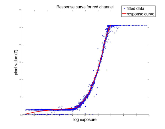
6. In the same figure, also include a plot of the log exposure for each of the pixels used as input to gsolve.m. To generate this plot, take the measured pixel value for each pixel and plot it against the sum of the recovered log irradiance and log exposure time, . The plot should look something like this:

3. Recover the HDR radiance map of the scene (3 Points)

Once you have recovered the camera response curve you are now ready to recover a radiance image from your sequence of exposures. You can recover you're the radiance map using the following equation

(3)

where P is the number of images that you captured in part 1). Here are some guidelines:

1. This can be a bit tricky to implement. Hint: The key here is that you will need to iterate over all possible pixel values. Use the Matlab 'find' function to get the indices of the pixels that correspond to a particular pixel value. Then use equation 3) to find the irradiance for those pixels. Repeat the procedure for each possible pixel value from 0-255;

2. You need to implement this equation separately for each color channel in the radiance image.

3. You can test out this code by downloading the response curve from here, and running your code on the memorial image sequence that you can download from Paul Debevec's website here. Your result should look something like this

4. Show a plot of the radiance image recovered from the AEB sequence you captured in part 1). What is the dynamic range of your scene? For example, i.e. the dynamic range of the memorial scene is nearly 10^6 or 1,000,000:1.

5. Implement a tone mapping algorithm to display your HDR image (5 Points)

The radiance map you recovered in part 3) likely has a much larger dynamic range than any electronic display device you will use to view the image. You now need to apply a simple global tone-mapping algorithm to your radiance image so that you can visualize the scene in a perceptually compelling way.

1. First just scale the brightness of each pixel uniformly so that all of the pixels fall in the range [0,1]. You will need to apply the following scaling algorithm to each color channel

(4)

where and are the maximum and minimum pixel values taken across all color channels. The image will likely look very dark because most of the display dynamic range will be used up by the pixels with higher radiance values Include a figure of this image.

2. Next apply a gamma curve to the image. To do this simply raise the irradiance of each pixel to the with an exponent of .

(5)

Play with different values for and report your results. Can you find a value that gives you visually pleasing results?

3. Lastly, try the global tone mapping operator from Reinhard '02 [2]. First you will need to convert the radiance image from color to grayscale. Note that you will first need to normalize the image using Eq. 4.

(6)

Then use the following equations to implement the tone mapping. We first calculate the log average exposure

(7)

Where the summation is over all of the pixels in the luminance image. Next scale the image according to:

(8)

Next apply the Reinhard tone-mapping operator:

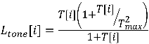(9)

Finally, define the scaling operator

and use this to scale each of the color channels in the radiance image. If the red, green, and blue channels of the radiance image are R, G, and B, form a new RGB image according to:

Experiment with different values for a. Try to find a value that gives visually pleasing results. A good starting point is . Include some figures of your tone-mapped images.

What to Submit:

Submit a zip file to the dropbox, which includes

1. A write-up document that explains what you did, what the results are, and what problems you encountered.

2. All code that you wrote, including the NativeCamera code running on the Tegra, and the Matlab code to evaluate the noise statistics.

3. The write-up should include all the figures that you were instructed to generate, and should answer all the questions posed in this document.

References:

1. Paul E. Debevec, Jitendra Malik, Recovering High Dynamic Range Radiance Maps from Photographs, SIGGRAPH 1997.

2. Erik Reinhard, Michael Stark, Peter Shirley, Jim Ferwerda, Photographics Tone Reproduction for Digital Images, SIGGRAPH 2002.